Calc spreadsheet file used in video: Right-click to download file
In a previous tutorial I wanted to get the total for a product in a table of sales figures, but what if I wanted a total for several products in the table?

This table is small, but if I had a lot of products it would be tedious to write a separate formula on each row to get it's total. Fortunatly there's no need to do this. I can write a formula and use the fill handle to copy it down the row to get all the product totals by using absolute and relative references. In the following example I'm building a table which multiplies the value in A2 by 1,2,3,4 and 5. The formula =A2*B4 is placed into Cell B5.

I can copy a formula across the cells by clicking cell B5 and dragging the fill handle across to F5, but it doesn't work in the other cells:

If I go to cell C5 and double click to view the formula, I can see why. When the formula was copied, the reference to the column in cell A2 moved to B when the formula was copied to C5, there's nothing in cell B2, so it was calculating 0*2 and yielding the answer 0.
The way to prevent this is to lock the column so it doesn't move when the formula is copied. This is done by placing a $ before the column reference, this is known as an absolute reference. I double-click in cell A5 and add a $ before the row reference:

I press Enter, then I drag the fill handle across to F5 again, and it works:
Double-click in cell F5 to view the formula and note that the reference to the column in cell A2 stayed locked on column A (absolute) while the other column reference moved from B to F (relative) when the formula was copied across the cells:

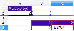
If I make a similar table with rows instead of columns, I will need an absolute reference to the row in cell A2 by placing a $ before the 2:

I click in C7 and pull the fill handle down to C11 and when I double-click on C11 I can see the row reference to Cell A2 stayed on 2 (absolute) while the row reference to the rows in column B changed to from 7 to ll (relative).

You can make both the row and column absolute by placing a $ before the row and column reference $A$2 and this would have worked in both of the above examples. But I used them separately in this case to demonstrate the principle.
You do not need to type the $ into the cell reference manually. After you type a cell reference in a formula press SHIFT F4 to insert $ before the column or row. Keep pressing SHIFT F4 repeatedly and it will toggle through all the possible combinations: row and column locked, row locked, column only locked, no lock.
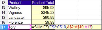
Now to apply this to the product totals in the first example:
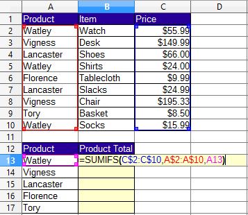

In the formula the rows were locked for the sum range and the criteria range so that the values wouldn't move when the formula was moved down to the other cells. the final parameter, which was the criteria, needs to change when copied to refer to the different products in column A. Double click cell B17 to reveal the formula and note that cell references in the last parameter (criteria) changed, but the other parameters stayed locked on the same cell ranges, press Esc to leave edit mode.
In this example I could have used an absolute reference to both rows and columns in the cell ranges and it would have worked:

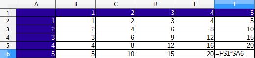
Here is a case where you really do need to make sure the absolute reference is to a row or a column and not both, another multiplication table:
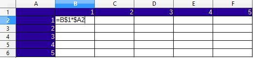
double-click F6 to reveal the formula and notice that the formula reads =F$1*$A6, in the first reference the row was locked and still refers to row one, but the column has changed to F because it wasn't locked, in the second reference, the column was locked, it still refers to column A, but the Row has now moved to 6.